* 본 포스팅은 머신러닝교과서를 참조하여 작성되었습니다.
* https://github.com/rickiepark/python-machine-learning-book-3rd-edition
GitHub - rickiepark/python-machine-learning-book-3rd-edition: <머신 러닝 교과서 3판>의 코드 저장소
<머신 러닝 교과서 3판>의 코드 저장소. Contribute to rickiepark/python-machine-learning-book-3rd-edition development by creating an account on GitHub.
github.com
8.2.1 단어를 특성 벡터로 변환
사이킷런에 구현된 CounterVectorizer 클래슬르 사용하여 각각의 문서에 있는 단어 카운트를 기반으로 BoW 모델을 만들 수 있다.
import numpy as np
from sklearn.feature_extraction.text import CountVectorizer
count = CountVectorizer()
docs = np.array([
    'The sun is shining',
    'The weather is sweet',
    'The sun is shining, the weather is sweet, and one and one is two'])
bag = count.fit_transform(docs)
print(count.vocabulary_)
>> {'the': 6, 'sun': 4, 'is': 1, 'shining': 3, 'weather': 8, 'sweet': 5, 'and': 0, 'one': 2, 'two': 7}print(bag.toarray())
>> [[0 1 0 1 1 0 1 0 0]
[0 1 0 0 0 1 1 0 1]
[2 3 2 1 1 1 2 1 1]]
8.2.2 tf-idf를 사용하여 단어 적합성 평가
텍스트 데이터를 분석할 때 클래스 레이블이 다른 문서에 같은 단어들이 나타나는 경우를 종종 보게 된다. 일반적으로 자주 등장하는 단어는 유용하거나 판별에 필요한 정보를 가지고 있지 않다.
특성 벡터에서 자주 등장하는 단어의 가중치를 낮추는 기법인 tf-idf(term frequency-inverse document frequency) 를 배워보자. tf-idf는 단어 빈도와 역문서 빈도(inverse document frequency)의 곱으로 정의된다.

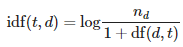
여기서 tf(t, d)는 단어 빈도이다. idf(t, d)는 역문서 빈도로 다음과 같이 계산한다.
from sklearn.feature_extraction.text import TfidfTransformer
tfidf = TfidfTransformer(use_idf=True,
                        norm='l2',
                        smooth_idf=True)
np.set_printoptions(precision=2)
print(tfidf.fit_transform(count.fit_transform(docs)).toarray())

>>  [[0.   0.43 0.   0.56 0.56 0.   0.43 0.   0.  ]
     [0.   0.43 0.   0.   0.   0.56 0.43 0.   0.56]
     [0.5  0.45 0.5  0.19 0.19 0.19 0.3  0.25 0.19]]
세 번째 문서에서 단어 'is'가 가장 많이 나타났기 때문에 단어 빈도가 가장 컸다. 동일한 특성 벡터를 tf-idf로 변환하면 단어 'is' 는 비교적 작은 tf-idf를 가진다(0.45). 이 단어는 첫 번째와 두 번째 문서에도 나타나므로 판별에 유용한 정보를 가지고 있지 않을 것이다.
수동으로 특성 벡터에 있는 각 단어의 tf-idf를 계산해 보면 TfidTransformer가 앞서 정의한 표준 tf-idf 공식과 조금 다르게 계산한다는 것을 알 수 있다. 사이킷런에 구현된 역문서 빈도 공식은 다음과 같다.

비슷하게 사이킷런에서 계산하는 tf-idf는 앞서 정의한 공식과 조금 다르다.
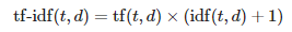
앞의 식에서 '+1'을 더한 것은 모든 문서에 등장하는 단어 가중치가 0이 되는 것(즉, idf(t,d)=log(1)=0)을 막기 위해서이다.
8.2.3 텍스트 데이터 정제
BoW 모델을 만들기 전에 첫 번째로 수행할 중요한 단계는 불필요한 문자를 삭제하여 텍스트 데이터를 정제하는 일이다.
랜덤하게 섞은 영화 리뷰 데이터셋의 첫 번째 문서에서 마지막 50개의 문자를 출력해 보자.
df.loc[0, 'review'][-50:]

>> 'is seven.<br /><br />Title (Brazil): Not Available'
정규 표현식(regular expression) 라이브러리 re를 사용하여 이모티콘 문자를 제외하고 모든 구두점 기호를 삭제한다.
import re
def preprocessor(text):
    text = re.sub('<[^>]*>', '', text)
    emoticons = re.findall('(?::|;|=)(?:-)?(?:\)|\(|D|P)',
                           text)
    text = (re.sub('[\W]+', ' ', text.lower()) +
            ' '.join(emoticons).replace('-', ''))
    return text
preprocessor(df.loc[0, 'review'][-50:])
>> 'is seven title brazil not available'
preprocessor("This :) is :( a test :-)!")
>> 'this is a test :) :( :)'
df['review'] = df['review'].apply(preprocessor)
8.2.4 문서를 토근으로 나누기
def tokenizer(text):
    return text.split()

tokenizer('runners like running and thus they run')

>> ['runners', 'like', 'running', 'and', 'thus', 'they', 'run']
포터 어간 추출(porter stemmer) 알고리즘
from nltk.stem.porter import PorterStemmer
porter = PorterStemmer()
def tokenizer_porter(text):
    return [porter.stem(word) for word in text.split()]

tokenizer_porter('runners like running and thus they run')

>> ['runner', 'like', 'run', 'and', 'thu', 'they', 'run']
앞 예를 보면 단어 'running'이 어간 'run'으로 바뀌었다.
BoW 모델을 사용하여 머신 러닝 모델을 훈련시키기 전에 불용어(stop-word)제거에 대해 알아보자. 불용어는 모든 종류의 텍스트에 아주 흔하게 등장하는 단어이다. 불용어 예로는 is, and, has, like 등이 있다. 불용어 제거는 tf-idf보다 기본 단어 빈도나 정규화된 단어 빈도를 사용할 때 더 유용하다. tf-idf에는 자주 등장하는 단어의 가중치가 이미 낮추어져 있다.
import nltk
nltk.download('stopwords')


from nltk.corpus import stopwords
stop = stopwords.words('english')

[w for w in tokenizer_porter('a runner likes running and runs a lot')[-10:] if w not in stop]
>> ['runner', 'like', 'run', 'run', 'lot']'소소하지만 소소하지 않은 개발 공부 > 머신 러닝 교과서' 카테고리의 다른 글
| 10.4 RANSAC을 사용하여 안정된 회귀 모델 훈련, python (0) | 2022.12.23 |
|---|---|
| 10.1 선형회귀, 머신러닝교과서, python (1) | 2022.12.22 |
| 7. 다양한 모델을 결합한 앙상블 학습, 머신러닝교과서, python (0) | 2022.12.19 |
| 6.2 k-겹 교차 검증을 사용한 모델 성능 평가 (0) | 2022.12.14 |
| 5.3 커널 PCA를 사용하여 비선형 매핑, 머신러닝교과서, python (0) | 2022.12.13 |